
Up to now we have been very fond of the unit square as domain, which is an appropriate choice for initial versions of a PDE solver. The strength of the finite element method, however, is its ease of handling domains with complex shapes. This section shows some methods that can be used to create different types of domains and meshes.
Domains of complex shape must normally be constructed in separate preprocessor programs. Two relevant preprocessors are Triangle for 2D domains and NETGEN for 3D domains.
DOLFIN has a few tools for creating various types of meshes over domains with simple shape: UnitInterval, UnitSquare, UnitCube, Interval, Rectangle, Box, UnitCircle, and UnitSphere.
Some of these names have been briefly met in previous sections. The hopefully self-explanatory code snippet below summarizes typical constructions of meshes with the aid of these tools:
# 1D domains
mesh = UnitInterval(20)     # 20 cells, 21 vertices
mesh = Interval(20, -1, 1)  # domain [-1,1]

# 2D domains (6x10 divisions, 120 cells, 77 vertices)
mesh = UnitSquare(6, 10)  # 'right' diagonal is default
# The diagonals can be right, left or crossed
mesh = UnitSquare(6, 10, 'left')
mesh = UnitSquare(6, 10, 'crossed')

# Domain [0,3]x[0,2] with 6x10 divisions and left diagonals
mesh = Rectangle(0, 0, 3, 2, 6, 10, 'left')

# 6x10x5 boxes in the unit cube, each box gets 6 tetrahedra:
mesh = UnitCube(6, 10, 5)

# Domain [-1,1]x[-1,0]x[-1,2] with 6x10x5 divisions
mesh = Box(-1, -1, -1, 1, 0, 2, 6, 10, 5)

# 10 divisions in radial directions
mesh = UnitCircle(10)
mesh = UnitSphere(10)
A mesh that is denser toward a boundary is often desired to increase
accuracy in that region. Given a mesh with uniformly spaced
coordinates  in
in ![[a,b]](_images/math/8ecbd1ba3da8f2adef66a63f2ab32c47e63fa734.png) , the coordinate transformation
, the coordinate transformation
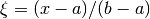 maps
maps  onto
onto ![\xi\in [0,1]](_images/math/9e0b480c03f67b2e25d5617b2722d3625a48abea.png) . A new mapping
. A new mapping
 , for some
  , stretches the mesh toward
  (
( ),
while
),
while  makes a stretching toward
  (
( ).
Mapping the
).
Mapping the ![\eta\in[0,1]](_images/math/07dec85e19693867b9e60a28b3f04f55fad1e6b2.png) coordinates back to gives new,
stretched coordinates,
coordinates back to gives new,
stretched coordinates,
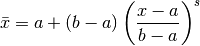
toward , or
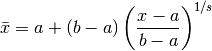
toward
One way of creating more complex geometries is to transform the
vertex coordinates in a rectangular mesh according to some formula.
Say we want to create a part of a hollow cylinder of  degrees,
with inner radius
degrees,
with inner radius  and outer radius
  . A standard mapping from polar
coordinates to Cartesian coordinates can be used to generate the
hollow cylinder. Given a rectangle in
. A standard mapping from polar
coordinates to Cartesian coordinates can be used to generate the
hollow cylinder. Given a rectangle in  space such that
 and
and  , the mapping

takes a point in the rectangular  geometry and maps it to a point
 in a hollow cylinder.
The corresponding Python code for first stretching the mesh and then mapping it onto a hollow cylinder looks as follows:
Theta = pi/2
a, b = 1, 5.0
nr = 10  # divisions in r direction
nt = 20  # divisions in theta direction
mesh = Rectangle(a, 0, b, 1, nr, nt, 'crossed')

# First make a denser mesh towards r=a
x = mesh.coordinates()[:,0]
y = mesh.coordinates()[:,1]
s = 1.3

def denser(x, y):
    return [a + (b-a)*((x-a)/(b-a))**s, y]

x_bar, y_bar = denser(x, y)
xy_bar_coor = numpy.array([x_bar, y_bar]).transpose()
mesh.coordinates()[:] = xy_bar_coor
plot(mesh, title='stretched mesh')

def cylinder(r, s):
    return [r*numpy.cos(Theta*s), r*numpy.sin(Theta*s)]

x_hat, y_hat = cylinder(x_bar, y_bar)
xy_hat_coor = numpy.array([x_hat, y_hat]).transpose()
mesh.coordinates()[:] = xy_hat_coor
plot(mesh, title='hollow cylinder')
interactive()
The result of calling denser and cylinder above is a list of two
vectors, with the and  coordinates, respectively.
Turning this list into a numpy array object results in a
coordinates, respectively.
Turning this list into a numpy array object results in a  array,
  being the number of vertices in the mesh. However,
mesh.coordinates() is by a convention an
being the number of vertices in the mesh. However,
mesh.coordinates() is by a convention an  array so we
need to take the transpose. The resulting mesh is displayed
in Figure Hollow cylinder generated by mapping a rectangular mesh, stretched toward the left side.
array so we
need to take the transpose. The resulting mesh is displayed
in Figure Hollow cylinder generated by mapping a rectangular mesh, stretched toward the left side.
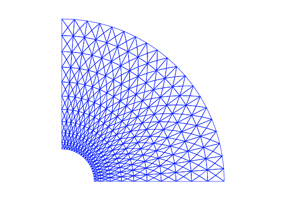
Hollow cylinder generated by mapping a rectangular mesh, stretched toward the left side
Setting boundary conditions in meshes created from mappings like the one illustrated above is most conveniently done by using a mesh function to mark parts of the boundary. The marking is easiest to perform before the mesh is mapped since one can then conceptually work with the sides in a pure rectangle. .. Stretch coordinates according to Mikael.