
FEniCS is a user-friendly tool for solving partial differential equations (PDEs). The goal of this tutorial is to get you started with FEniCS through a series of simple examples that demonstrate
- how to define the PDE problem in terms of a variational problem,
- how to define simple domains,
- how to deal with Dirichlet, Neumann, and Robin conditions,
- how to deal with variable coefficients,
- how to deal with domains built of several materials (subdomains),
- how to compute derived quantities like the flux vector field or a functional of the solution,
- how to quickly visualize the mesh, the solution, the flux, etc.,
- how to solve nonlinear PDEs in various ways,
- how to deal with time-dependent PDEs,
- how to set parameters governing solution methods for linear systems,
- how to create domains of more complex shape.
The mathematics of the illustrations is kept simple to better focus on FEniCS functionality and syntax. This means that we mostly use the Poisson equation and the time-dependent diffusion equation as model problems, often with input data adjusted such that we get a very simple solution that can be exactly reproduced by any standard finite element method over a uniform, structured mesh. This latter property greatly simplifies the verification of the implementations. Occasionally we insert a physically more relevant example to remind the reader that changing the PDE and boundary conditions to something more real might often be a trivial task.
FEniCS may seem to require a thorough understanding of the abstract mathematical version of the finite element method as well as familiarity with the Python programming language. Nevertheless, it turns out that many are able to pick up the fundamentals of finite elements and Python programming as they go along with this tutorial. Simply keep on reading and try out the examples. You will be amazed of how easy it is to solve PDEs with FEniCS!
Reading this tutorial obviously requires access to a machine where the FEniCS software is installed. The section Installing FEniCS explains briefly how to install the necessary tools.
All the examples discussed in the following are available as executable Python source code files in a directory tree.
Our first example regards the Poisson problem,
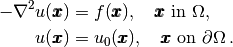
Here,  is the unknown function,
  is a
prescribed function,
is a
prescribed function,  is the Laplace operator (also
often written as
is the Laplace operator (also
often written as  ),
),  is the spatial domain, and
 is the boundary of . A stationary PDE like
this, together with a complete set of boundary conditions, constitute
a boundary-value problem, which must be precisely stated before
it makes sense to start solving it with FEniCS.
is the boundary of . A stationary PDE like
this, together with a complete set of boundary conditions, constitute
a boundary-value problem, which must be precisely stated before
it makes sense to start solving it with FEniCS.
In two space dimensions with coordinates  and
and  , we can write out
the Poisson equation as
, we can write out
the Poisson equation as
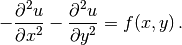
The unknown  is now a function of two variables,
  , defined
over a two-dimensional domain .
, defined
over a two-dimensional domain .
The Poisson equation arises in numerous physical contexts, including heat conduction, electrostatics, diffusion of substances, twisting of elastic rods, inviscid fluid flow, and water waves. Moreover, the equation appears in numerical splitting strategies of more complicated systems of PDEs, in particular the Navier-Stokes equations.
Solving a physical problem with FEniCS consists of the following steps:
- Identify the PDE and its boundary conditions.
- Reformulate the PDE problem as a variational problem.
- Make a Python program where the formulas in the variational problem are coded, along with definitions of input data such as
,
, and a mesh for the spatial domain
- Add statements in the program for solving the variational problem, computing derived quantities such as
, and visualizing the results.
We shall now go through steps 2–4 in detail. The key feature of FEniCS is that steps 3 and 4 result in fairly short code, while most other software frameworks for PDEs require much more code and more technically difficult programming.
FEniCS makes it easy to solve PDEs if finite elements are used for discretization in space and the problem is expressed as a variational problem. Readers who are not familiar with variational problems will get a brief introduction to the topic in this tutorial, but getting and reading a proper book on the finite element method in addition is encouraged. The section Books on the Finite Element Method contains a list of some suitable books.
The core of the recipe for turning a PDE into a variational problem
is to multiply the PDE by a function  , integrate the resulting
equation over , and perform integration by parts of terms with
second-order derivatives. The function which multiplies the PDE
is in the mathematical finite element literature
called a test function. The unknown function to be approximated
is referred to
as a trial function. The terms test and trial function are used
in FEniCS programs too.
Suitable
function spaces must be specified for the test and trial functions.
For standard PDEs arising in physics and mechanics such spaces are
well known.
, integrate the resulting
equation over , and perform integration by parts of terms with
second-order derivatives. The function which multiplies the PDE
is in the mathematical finite element literature
called a test function. The unknown function to be approximated
is referred to
as a trial function. The terms test and trial function are used
in FEniCS programs too.
Suitable
function spaces must be specified for the test and trial functions.
For standard PDEs arising in physics and mechanics such spaces are
well known.
In the present case, we first multiply the Poisson equation
by the test function and integrate,
(1)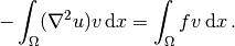
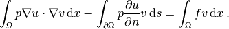
Then we apply integration by parts to the integrand with second-order derivatives,
(2)
where  is the derivative of in the outward normal direction at
the boundary.
The test function is required to vanish on the parts of the
boundary where is known, which in the present problem implies that
is the derivative of in the outward normal direction at
the boundary.
The test function is required to vanish on the parts of the
boundary where is known, which in the present problem implies that
 on the whole boundary .
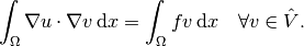
The second term on the right-hand side of the last equation therefore
vanishes. It then follows that
on the whole boundary .
The second term on the right-hand side of the last equation therefore
vanishes. It then follows that
(3)
This equation is supposed to hold
for all in some function space  . The trial function
lies in some (possibly different) function space
. The trial function
lies in some (possibly different) function space  .
We say that the last equation is the weak form of the original
boundary value problem consisting of the PDE
.
We say that the last equation is the weak form of the original
boundary value problem consisting of the PDE  and the
boundary condition
and the
boundary condition  .
.
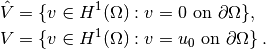
The proper statement of
our variational problem now goes as follows:
Find  such that
(4)
The test and trial spaces  and are in the present
problem defined as
and are in the present
problem defined as
In short,
 is the mathematically well-known Sobolev space containing
functions such that
is the mathematically well-known Sobolev space containing
functions such that  and
and  have finite integrals over
. The solution of the underlying
PDE
must lie in a function space where also the derivatives are continuous,
but the Sobolev space allows functions with discontinuous
derivatives.
This weaker continuity requirement of in the variational
statement,
caused by the integration by parts, has
great practical consequences when it comes to constructing
finite elements.
have finite integrals over
. The solution of the underlying
PDE
must lie in a function space where also the derivatives are continuous,
but the Sobolev space allows functions with discontinuous
derivatives.
This weaker continuity requirement of in the variational
statement,
caused by the integration by parts, has
great practical consequences when it comes to constructing
finite elements.
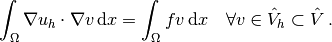
To solve the Poisson equation numerically, we need to transform the
continuous variational problem
to a discrete variational
problem. This is done by introducing finite-dimensional test and
trial spaces, often denoted as
 and
and  . The
discrete variational problem reads:
Find
. The
discrete variational problem reads:
Find  such that
(5)
The choice of  and
and  follows directly from the
kind of finite elements we want to apply in our problem. For example,
choosing the well-known linear triangular element with three nodes
implies that
follows directly from the
kind of finite elements we want to apply in our problem. For example,
choosing the well-known linear triangular element with three nodes
implies that
 and are the spaces of all piecewise linear functions
over a mesh of triangles,
where the functions in
are zero on the boundary
and those in equal on the boundary.
and are the spaces of all piecewise linear functions
over a mesh of triangles,
where the functions in
are zero on the boundary
and those in equal on the boundary.
The mathematics literature on variational problems writes  for
the solution of the discrete problem and for the solution of the
continuous problem. To obtain (almost) a one-to-one relationship
between the mathematical formulation of a problem and the
corresponding FEniCS program, we shall use for the solution of
the discrete problem and
for
the solution of the discrete problem and for the solution of the
continuous problem. To obtain (almost) a one-to-one relationship
between the mathematical formulation of a problem and the
corresponding FEniCS program, we shall use for the solution of
the discrete problem and  for the exact solution of the
continuous problem, if we need to explicitly distinguish
between the two. In most cases, we will introduce the PDE problem with
as unknown, derive a variational equation
for the exact solution of the
continuous problem, if we need to explicitly distinguish
between the two. In most cases, we will introduce the PDE problem with
as unknown, derive a variational equation  with
with  and
and  , and then simply discretize the problem by saying
that we choose finite-dimensional spaces for and . This
restriction of implies that becomes a discrete finite element
function. In practice, this means that we turn our PDE problem into a
continuous variational problem, create a mesh and specify an element
type, and then let correspond to this mesh and element choice.
Depending upon whether is infinite- or finite-dimensional,
will be the exact or approximate solution.
, and then simply discretize the problem by saying
that we choose finite-dimensional spaces for and . This
restriction of implies that becomes a discrete finite element
function. In practice, this means that we turn our PDE problem into a
continuous variational problem, create a mesh and specify an element
type, and then let correspond to this mesh and element choice.
Depending upon whether is infinite- or finite-dimensional,
will be the exact or approximate solution.
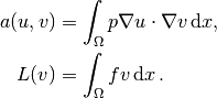
It turns out to be convenient to introduce the following unified notation for linear weak forms:
In the present problem we have that
From the mathematics literature,
 is known as a bilinear form and
  as a
linear form.
We shall in every linear problem we solve identify the terms with the
unknown and collect them in , and similarly collect
all terms with only known functions in . The formulas for
as a
linear form.
We shall in every linear problem we solve identify the terms with the
unknown and collect them in , and similarly collect
all terms with only known functions in . The formulas for  and
and
 are then coded directly in the program.
To summarize, before making a FEniCS program for solving a PDE, we must first perform two steps:
- Turn the PDE problem into a discrete variational problem: find
such that
.
- Specify the choice of spaces (
The test problem so far has a general domain and general functions
and . For our first implementation we must decide on specific
choices of , , and .
It will be wise to construct a specific problem where we can easily
check that the computed solution is correct. Let us start with
specifying an exact solution
(6)
on some 2D domain. By inserting eq:ref:tut:poisson1:impl:uex in
our Poisson problem, we find that  is a solution if

regardless of the shape of the domain. We choose here, for simplicity, the domain to be the unit square,
![\Omega = [0,1]\times [0,1] .](_images/math/95a8c5e0238278eec467d80802df9f655ca2fc04.png)
The reason for specifying the solution eq:ref:tut:poisson1:impl:uex
is that the finite element method, with a rectangular domain uniformly
partitioned into linear triangular elements, will exactly reproduce a
second-order polynomial at the vertices of the cells, regardless of
the size of the elements. This property allows us to verify the
implementation by comparing the computed solution, called in this
document (except when setting up the PDE problem), with the exact
solution, denoted by  : should equal
 to machine precision emph{at the nodes}.
Test problems with this property will be frequently constructed
throughout this tutorial.
to machine precision emph{at the nodes}.
Test problems with this property will be frequently constructed
throughout this tutorial.
A FEniCS program for solving the Poisson equation in 2D
with the given choices
of , , and may look as follows:
"""
FEniCS tutorial demo program: Poisson equation with Dirichlet conditions.
Simplest example of computation and visualization with FEniCS.

-Laplace(u) = f on the unit square.
u = u0 on the boundary.
u0 = u = 1 + x^2 + 2y^2, f = -6.
"""

from dolfin import *

# Create mesh and define function space
mesh = UnitSquare(6, 4)
#mesh = UnitCube(6, 4, 5)
V = FunctionSpace(mesh, 'Lagrange', 1)

# Define boundary conditions
u0 = Expression('1 + x[0]*x[0] + 2*x[1]*x[1]')

def u0_boundary(x, on_boundary):
    return on_boundary

bc = DirichletBC(V, u0, u0_boundary)

# Define variational problem
u = TrialFunction(V)
v = TestFunction(V)
f = Constant(-6.0)
a = inner(nabla_grad(u), nabla_grad(v))*dx
L = f*v*dx

# Compute solution
u = Function(V)
solve(a == L, u, bc)

# Plot solution and mesh
plot(u)
plot(mesh)

# Dump solution to file in VTK format
file = File('poisson.pvd')
file << u

# Hold plot
interactive()
The complete code can be found in the file d1_p2D.py in the directory stationary/poisson.
We shall now dissect this FEniCS program in detail. The program is written in the Python programming language. You may either take a quick look at the official Python tutorial to pick up the basics of Python if you are unfamiliar with the language, or you may learn enough Python as you go along with the examples in the present tutorial. The latter strategy has proven to work for many newcomers to FEniCS. (The requirement of using Python and an abstract mathematical formulation of the finite element problem may seem difficult for those who are unfamiliar with these topics. However, the amount of mathematics and Python that is really demanded to get you productive with FEniCS is quite limited. And Python is an easy-to-learn language that you certainly will love and use far beyond FEniCS programming.) the section Books on Python lists some relevant Python books.
The listed FEniCS program defines a finite element mesh, the discrete
function spaces and corresponding to this mesh and
the element type, boundary conditions
for (the function ), , and .
Thereafter, the unknown
trial function is computed. Then we can investigate visually or
analyze the computed values.
The first line in the program,
from dolfin import *
imports the key classes UnitSquare, FunctionSpace, Function, and so forth, from the DOLFIN library. All FEniCS programs for solving PDEs by the finite element method normally start with this line. DOLFIN is a software library with efficient and convenient C++ classes for finite element computing, and dolfin is a Python package providing access to this C++ library from Python programs. You can think of FEniCS as an umbrella, or project name, for a set of computational components, where DOLFIN is one important component for writing finite element programs. The from dolfin import * statement imports other components too, but newcomers to FEniCS programming do not need to care about this.
The statement
mesh = UnitSquare(6, 4)
defines a uniform finite element mesh over the unit square
![[0,1]\times [0,1]](_images/math/ac8e6ab5cdf1c6a6e37ea0439ed75612939e0abb.png) . The mesh consists of cells,
which are triangles with
straight sides. The parameters 6 and 4 tell that the square is
first divided into
. The mesh consists of cells,
which are triangles with
straight sides. The parameters 6 and 4 tell that the square is
first divided into  rectangles, and then each rectangle
is divided into two triangles. The total number of triangles
then becomes 48. The total number of vertices in this mesh is
rectangles, and then each rectangle
is divided into two triangles. The total number of triangles
then becomes 48. The total number of vertices in this mesh is
 .
DOLFIN offers some classes for creating meshes over
very simple geometries. For domains of more complicated shape one needs
to use a separate preprocessor program to create the mesh.
The FEniCS program will then read the mesh from file.
.
DOLFIN offers some classes for creating meshes over
very simple geometries. For domains of more complicated shape one needs
to use a separate preprocessor program to create the mesh.
The FEniCS program will then read the mesh from file.
Having a mesh, we can define a discrete function space V over this mesh:
V = FunctionSpace(mesh, 'Lagrange', 1)
The second argument reflects the type of element, while the third argument is the degree of the basis functions on the element.
The type of element is here “Lagrange”, implying the
standard Lagrange family of elements.
(Some FEniCS programs use 'CG', for Continuous Galerkin,
as a synonym for 'Lagrange'.)
With degree 1, we simply get the standard linear Lagrange element,
which is a triangle
with nodes at the three vertices.
Some finite element practitioners refer to this element as the
“linear triangle”.
The computed will be continuous and linearly varying in and over
each cell in the mesh.
Higher-degree polynomial approximations over each cell are
trivially obtained by increasing the third parameter in
FunctionSpace. Changing the second parameter to 'DG' creates a
function space for discontinuous Galerkin methods.
In mathematics, we distinguish between the trial and test
spaces and . The only difference in the present problem
is the boundary conditions. In FEniCS we do not specify the boundary
conditions as part of the function space, so it is sufficient to work
with one common space V for the and trial and test functions in the
program:
u = TrialFunction(V)
v = TestFunction(V)
The next step is to specify the boundary condition: on
. This is done by
bc = DirichletBC(V, u0, u0_boundary)
where u0 is an instance holding the values,
and u0_boundary is a function (or object) describing whether a point lies
on the boundary where is specified.
Boundary conditions
of the type are known as Dirichlet conditions, and also
as essential boundary conditions in a finite element context.
Naturally, the name of the DOLFIN class holding the information about
Dirichlet boundary conditions is DirichletBC.
The u0 variable refers to an Expression object, which is used to represent a mathematical function. The typical construction is
u0 = Expression(formula)
where formula is a string containing the mathematical expression.
This formula is
written with C++ syntax (the expression is
automatically turned into an efficient, compiled
C++ function, see the section User-Defined Functions for
details on the syntax). The independent variables in the function
expression are supposed to be available
as a point vector x, where the first element x[0]
corresponds to the coordinate, the second element x[1]
to the coordinate, and (in a three-dimensional problem)
x[2] to the  coordinate. With our choice of
 , the formula string must be written
as 1 + x[0]*x[0] + 2*x[1]*x[1]:
, the formula string must be written
as 1 + x[0]*x[0] + 2*x[1]*x[1]:
u0 = Expression('1 + x[0]*x[0] + 2*x[1]*x[1]')
The information about where to apply the u0 function as boundary condition is coded in a function u0_boundary:
def u0_boundary(x, on_boundary):
    return on_boundary
A function like u0_boundary for marking the boundary must
return
a boolean value: True if the given point
x lies on the Dirichlet boundary and
False otherwise.
The argument on_boundary is True if x is on
the physical boundary of the mesh, so in the present case, where
we are supposed to return True for all points on
the boundary, we can just return the supplied value of
on_boundary.
The u0_boundary function will be called
for every discrete point in the mesh, which allows us to have boundaries
where are known also inside the domain, if desired.
One can also omit the on_boundary argument, but in that case we need to test on the value of the coordinates in x:
def u0_boundary(x):
    return x[0] == 0 or x[1] == 0 or x[0] == 1 or x[1] == 1
As for the formula in Expression objects, x in the u0_boundary function represents a point in space with coordinates x[0], x[1], etc. Comparing floating-point values using an exact match test with == is not good programming practice, because small round-off errors in the computations of the x values could make a test x[0] == 1 become false even though x lies on the boundary. A better test is to check for equality with a tolerance:
def u0_boundary(x):
    tol = 1E-15
    return abs(x[0]) < tol or \
           abs(x[1]) < tol or \
           abs(x[0] - 1) < tol or \
           abs(x[1] - 1) < tol
Before defining and we have to specify the function:
f = Expression('-6')
When is constant over the domain, f can be
more efficiently represented as a Constant object:
f = Constant(-6.0)
Now we have all the objects we need in order to specify this problem’s
and :
a = inner(nabla_grad(u), nabla_grad(v))*dx
L = f*v*dx
In essence, these two lines specify the PDE to be solved.
Note the very close correspondence between the Python syntax
and the mathematical formulas  and
and
 .
This is a key strength of FEniCS: the formulas in the variational
formulation translate directly to very similar Python code, a feature
that makes it easy to specify PDE problems with lots of PDEs and
complicated terms in the equations.
The language used to express weak forms is called UFL (Unified Form Language)
and is an integral part of FEniCS.
.
This is a key strength of FEniCS: the formulas in the variational
formulation translate directly to very similar Python code, a feature
that makes it easy to specify PDE problems with lots of PDEs and
complicated terms in the equations.
The language used to express weak forms is called UFL (Unified Form Language)
and is an integral part of FEniCS.
Instead of nabla_grad we could also just have written grad in the examples in this tutorial. However, when taking gradients of vector fields, grad and nabla_grad differ. The latter is consistent with the tensor algebra commonly used to derive vector and tensor PDEs, where the “nabla” acts as a vector operator, and therefore this author prefers to always use nabla_grad.
Having a and L defined, and information about essential (Dirichlet) boundary conditions in bc, we can compute the solution, a finite element function u, by
u = Function(V)
solve(a == L, u, bc)
Some prefer to replace a and L by an equation variable, which is accomplished by this equivalent code:
equation = inner(nabla_grad(u), nabla_grad(v))*dx == f*v*dx
u = Function(V)
solve(equation, u, bc)
Note that we first defined the variable u as a
TrialFunction and used it to represent the unknown in the form
a. Thereafter, we redefined u to be a Function
object representing the solution, i.e., the computed finite element
function . This redefinition of the variable u is possible
in Python and often done in FEniCS applications. The two types of
objects that u refers to are equal from a mathematical point of
view, and hence it is natural to use the same variable name for both
objects. In a program, however, TrialFunction objects must
always be used for the unknowns in the problem specification (the form
a), while Function objects must be used for quantities
that are computed (known).
The simplest way of quickly looking at u and the mesh is to say
plot(u)
plot(mesh)
interactive()
The interactive() call is necessary for the plot to remain on the
screen. With the left, middle, and right
mouse buttons you can rotate, translate, and zoom
(respectively) the plotted surface to better examine what the solution looks
like.
Figures Plot of the solution in the first FEniCS example and Plot of the mesh in the first FEniCS example
display the resulting function and the finite element mesh, respectively.
It is also possible to dump the computed solution to file, e.g., in the VTK format:
file = File('poisson.pvd')
file << u
The poisson.pvd file can now be loaded into any front-end to VTK, say ParaView or VisIt. The plot function is intended for quick examination of the solution during program development. More in-depth visual investigations of finite element solutions will normally benefit from using highly professional tools such as ParaView and VisIt.
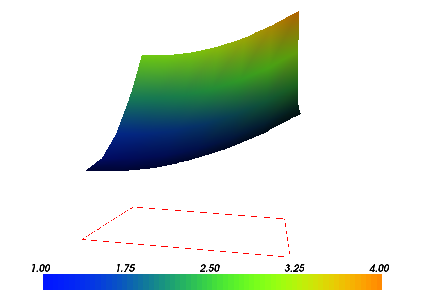
Plot of the solution in the first FEniCS example
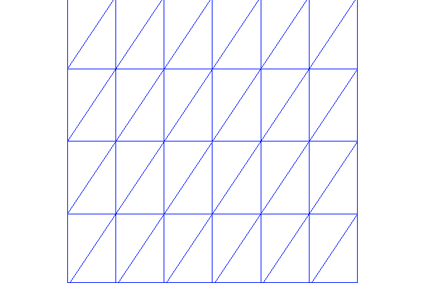
Plot of the mesh in the first FEniCS example
The next three sections deal with some technicalities about specifying the solution method for linear systems (so that you can solve large problems) and examining array data from the computed solution (so that you can check that the program is correct). These technicalities are scattered around in forthcoming programs. However, the impatient reader who is more interested in seeing the previous program being adapted to a real physical problem, and play around with some interesting visualizations, can safely jump to the section Solving a Real Physical Problem. Information in the intermediate sections can be studied on demand.
Sparse LU decomposition (Gaussian elimination) is used by default to solve linear systems of equations in FEniCS programs. This is a very robust and recommended method for a few thousand unknowns in the equation system, and may hence be the method of choice in many 2D and smaller 3D problems. However, sparse LU decomposition becomes slow and memory demanding in large problems. This fact forces the use of iterative methods, which are faster and require much less memory.
Preconditioned Krylov solvers is a type of popular iterative methods that are easily accessible in FEniCS programs. The Poisson equation results in a symmetric, positive definite coefficient matrix, for which the optimal Krylov solver is the Conjugate Gradient (CG) method. Incomplete LU factorization (ILU) is a popular and robust all-round preconditioner, so let us try the CG–ILU pair:
solve(a == L, u, bc)
      solver_parameters={'linear_solver': 'cg',
                         'preconditioner': 'ilu'})
# Alternative syntax
solve(a == L, u, bc,
      solver_parameters=dict(linear_solver='cg',
                             preconditioner='ilu'))
the section Linear Solvers and Preconditioners lists the most popular choices of Krylov solvers and preconditioners available in FEniCS
The actual CG and ILU implementations that are brought into action depends on the choice of linear algebra package. FEniCS interfaces several linear algebra packages, called linear algebra backends in FEniCS terminology. PETSc is the default choice if DOLFIN is compiled with PETSc, otherwise uBLAS. Epetra (Trilinos) and MTL4 are two other supported backends. Which backend to apply can be controlled by setting
parameters['linear_algebra_backend'] = backendname
where backendname is a string, either 'PETSc', 'uBLAS', 'Epetra', or 'MTL4'. All these backends offer high-quality implementations of both iterative and direct solvers for linear systems of equations.
A common platform for FEniCS users is Ubuntu Linux. The FEniCS distribution for Ubuntu contains PETSc, making this package the default linear algebra backend. The default solver is sparse LU decomposition ('lu'), and the actual software that is called is then the sparse LU solver from UMFPACK (which PETSc has an interface to).
We will normally like to control the tolerance in the stopping criterion and the maximum number of iterations when running an iterative method. Such parameters can be set by accessing the global parameter database, which is called parameters and which behaves as a nested dictionary. Write
info(parameters, True)
to list all parameters and their default values in the database. The nesting of parameter sets is indicated through indentation in the output from info. According to this output, the relevant parameter set is named 'krylov_solver', and the parameters are set like this:
prm = parameters['krylov_solver'] # short form
prm['absolute_tolerance'] = 1E-10
prm['relative_tolerance'] = 1E-6
prm['maximum_iterations'] = 1000
Stopping criteria for Krylov solvers usually involve the norm of the residual, which must be smaller than the absolute tolerance parameter or smaller than the relative tolerance parameter times the initial residual.
To see the number of actual iterations to reach the stopping criterion, we can insert
set_log_level(PROGRESS)
# or
set_log_level(DEBUG)
A message with the equation system size, solver type, and number of iterations arises from specifying the argument PROGRESS, while DEBUG results in more information, including CPU time spent in the various parts of the matrix assembly and solve process.
The complete solution process with control of the solver parameters now contains the statements
prm = parameters['krylov_solver'] # short form
prm['absolute_tolerance'] = 1E-10
prm['relative_tolerance'] = 1E-6
prm['maximum_iterations'] = 1000
set_log_level(PROGRESS)

solve(a == L, u, bc,
      solver_parameters={'linear_solver': 'cg',
                         'preconditioner': 'ilu'})
The demo program d2_p2D.py in the stationary/poisson directory incorporates the above shown control of the linear solver and precnditioner, but is otherwise similar to the previous d1_p2D.py program.
We remark that default values for the global parameter database can be defined in an XML file, see the example file dolfin_parameters.xml in the directory stationary/poisson. If such a file is found in the directory where a FEniCS program is run, this file is read and used to initialize the parameters object. Otherwise, the file .config/fenics/dolfin_parameters.xml in the user’s home directory is read, if it exists. The XML file can also be in gzip’ed form with the extension .xml.gz.
The solve(a == L, u, bc) call is just a compact syntax alternative to a slightly more comprehensive specification of the variational equation and the solution of the associated linear system. This alternative syntax is used in a lot of FEniCS applications and will also be used later in this tutorial, so we show it already now:
u = Function(V)
problem = LinearVariationalProblem(a, L, u, bc)
solver  = LinearVariationalSolver(problem)
solver.solve()
Many objects have an attribute parameters corresponding to a parameter set in the global parameters database, but local to the object. Here, solver.parameters play that role. Setting the CG method with ILU preconditiong as solution method and specifying solver-specific parameters can be done like this:
solver.parameters['linear_solver'] = 'cg'
solver.parameters['preconditioner'] = 'ilu'
cg_prm = solver.parameters['krylov_solver'] # short form
cg_prm['absolute_tolerance'] = 1E-7
cg_prm['relative_tolerance'] = 1E-4
cg_prm['maximum_iterations'] = 1000
Calling info(solver.parameters, True) lists all the available parameter sets with default values for each parameter. Settings in the global parameters database are propagated to parameter sets in individual objects, with the possibility of being overwritten as done above.
The d3_p2D.py program modifies the d2_p2D.py file to incorporate objects for the variational problem and solver.
We know that, in the particular boundary-value problem of the section Implementation (1), the computed solution should equal the
exact solution at the vertices of the cells. An important extension
of our first program is therefore to examine the computed values of
the solution, which is the focus of the present section.
A finite element function like is expressed as a linear combination
of basis functions  , spanning the space :
(7)
By writing solve(a == L, u, bc) in the program, a linear system
will be formed from and , and this system is solved for the
 values. The values are known
as degrees of freedom of . For Lagrange elements (and many other
element types)  is simply the value of at the node
with global number
is simply the value of at the node
with global number  .
(The nodes and cell vertices coincide for linear Lagrange elements, while
for higher-order elements there may be additional nodes at
the facets and in the interior of cells.)
.
(The nodes and cell vertices coincide for linear Lagrange elements, while
for higher-order elements there may be additional nodes at
the facets and in the interior of cells.)
Having u represented as a Function object,
we can either evaluate u(x) at any vertex x in the mesh,
or we can grab all the values
 directly by
u_nodal_values = u.vector()
The result is a DOLFIN Vector object, which is basically an encapsulation of the vector object used in the linear algebra package that is used to solve the linear system arising from the variational problem. Since we program in Python it is convenient to convert the Vector object to a standard numpy array for further processing:
u_array = u_nodal_values.array()
With numpy arrays we can write “MATLAB-like” code to analyze the data. Indexing is done with square brackets: u_array[i], where the index i always starts at 0.
 numpy array,
 being the number of vertices in the mesh and
  being
the number of space dimensions,
being
the number of space dimensions,Writing print mesh dumps a short, “pretty print” description of the mesh (print mesh actually displays the result of str(mesh)`, which defines the pretty print):
<Mesh of topological dimension 2 (triangles) with
16 vertices and 18 cells, ordered>
All mesh objects are of type Mesh so typing the command pydoc dolfin.Mesh in a terminal window will give a list of methods (that is, functions in a class) that can be called through any Mesh object. In fact, pydoc dolfin.X shows the documentation of any DOLFIN name X.
Writing out the solution on the screen can now be done by a simple loop:
coor = mesh.coordinates()
if mesh.num_vertices() == len(u_array):
    for i in range(mesh.num_vertices()):
        print 'u(%8g,%8g) = %g' % (coor[i][0], coor[i][1], u_array[i])
The beginning of the output looks like this:
u(       0,       0) = 1
u(0.166667,       0) = 1.02778
u(0.333333,       0) = 1.11111
u(     0.5,       0) = 1.25
u(0.666667,       0) = 1.44444
u(0.833333,       0) = 1.69444
u(       1,       0) = 2
For Lagrange elements of degree higher than one, the vertices do not correspond to all the nodal points and the if-test fails.
For verification purposes we want to compare the values of the computed u at the nodes (given by u_array) with the exact solution u0 evaluated at the nodes. The difference between the computed and exact solution should be less than a small tolerance at all the nodes. The Expression object u0 can be evaluated at any point x by calling u0(x). Specifically, u0(coor[i]) returns the value of u0 at the vertex or node with global number i.
Alternatively, we can make a finite element field u_e, representing
the exact solution, whose values at the nodes are given by the
u0 function. With mathematics,  , where
 ,
,  being the coordinates of node number
  .
This process is known as interpolation.
FEniCS has a function for performing the operation:
.
This process is known as interpolation.
FEniCS has a function for performing the operation:
u_e = interpolate(u0, V)
The maximum error can now be computed as
u_e_array = u_e.vector().array()
print 'Max error:', numpy.abs(u_e_array - u_array).max()
The value of the error should be at the level of the machine precision
( ).
).
To demonstrate the use of point evaluations of Function objects, we write out the computed u at the center point of the domain and compare it with the exact solution:
center = (0.5, 0.5)
print 'numerical u at the center point:',  u(center)
print 'exact     u at the center point:', u0(center)
Trying a  mesh, the output from the
previous snippet becomes
mesh, the output from the
previous snippet becomes
numerical u at the center point: [ 1.83333333]
exact     u at the center point: [ 1.75]
The discrepancy is due to the fact that the center point is not a node in this particular mesh, but a point in the interior of a cell, and u varies linearly over the cell while u0 is a quadratic function.
We have seen how to extract the nodal values in a numpy array.
If desired, we can adjust the nodal values too. Say we want to
normalize the solution such that  . Then we
must divide all values
by
. Then we
must divide all values
by  . The following snippet performs the task:
max_u = u_array.max()
u_array /= max_u
u.vector()[:] = u_array
u.vector().set_local(u_array)  # alternative
print u.vector().array()
That is, we manipulate u_array as desired, and then we insert this array into u‘s Vector object. The /= operator implies an in-place modification of the object on the left-hand side: all elements of the u_array are divided by the value max_u. Alternatively, one could write u_array = u_array/max_u, which implies creating a new array on the right-hand side and assigning this array to the name u_array.
A call like u.vector().array() returns a copy of the data in u.vector(). One must therefore never perform assignments like u.vector.array()[:] = ..., but instead extract the numpy array (i.e., a copy), manipulate it, and insert it back with u.vector()[:] = `` or ``u.set_local(...).
All the code in this subsection can be found in the file d4_p2D.py in the stationary/poisson directory. We have commented out the plotting statements in this version of the program, but if you want plotting to happen, make sure that interactive is called at the very end of the program.
Perhaps you are not particularly amazed by viewing the simple surface
of in the test problem from the section Implementation (1).
However, solving a real physical problem
with a more interesting and amazing solution on the screen is only a
matter of specifying a more exciting domain, boundary condition,
and/or right-hand side .
One possible physical problem regards the deflection
 of an elastic circular membrane
with radius
of an elastic circular membrane
with radius  , subject to a localized perpendicular pressure
force, modeled as a Gaussian function.
The appropriate PDE model is
, subject to a localized perpendicular pressure
force, modeled as a Gaussian function.
The appropriate PDE model is

with
Here,  is the tension in the membrane (constant),
  is the external
pressure load,
is the external
pressure load,
 the amplitude of the pressure,
  the localization of
the Gaussian pressure function, and
the localization of
the Gaussian pressure function, and  the “width” of this
function. The boundary of the membrane has no
deflection, implying
the “width” of this
function. The boundary of the membrane has no
deflection, implying  as boundary condition.
For scaling and verification it is convenient to simplify the problem
to find an analytical solution. In the limit  ,
,
 , which allows us to integrate an axi–symmetric
version of the equation in the radial coordinate
, which allows us to integrate an axi–symmetric
version of the equation in the radial coordinate ![r\in [0,R]](_images/math/161bb3c87f6519e8327671e9a73c1acc27a0940f.png) and
obtain
and
obtain  . This result gives
a rough estimate of the characteristic size of the deflection:
. This result gives
a rough estimate of the characteristic size of the deflection:
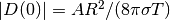 , which can be used to scale the deflecton.
With as characteristic length scale, we can derive the equivalent
dimensionless problem on the unit circle,
, which can be used to scale the deflecton.
With as characteristic length scale, we can derive the equivalent
dimensionless problem on the unit circle,
(8)
with  on the boundary and with
(9)
end{equation}
For notational convenience we have dropped introducing new symbols
for the scaled
coordinates in (9).
Now  is related to
  through
 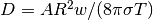 .
.
Let us list the modifications of the d1_p2D.py program that are needed to solve this membrane problem:
- Initialize
,
, and
- create a mesh over the unit circle,
- make an expression object for the scaled pressure function
- define the a and L formulas in the variational problem for
- plot the mesh,
- write out the maximum real deflection
Some suitable values of , , , , , and are
T = 10.0  # tension
A = 1.0   # pressure amplitude
R = 0.3   # radius of domain
theta = 0.2
x0 = 0.6*R*cos(theta)
y0 = 0.6*R*sin(theta)
sigma = 0.025
A mesh over the unit circle can be created by
mesh = UnitCircle(n)
where n is the typical number of elements in the radial direction.
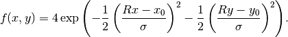
The function is represented by an Expression object. There
are many physical parameters in the formula for that enter the
expression string and these parameters must have their values set
by keyword arguments:
f = Expression('4*exp(-0.5*(pow((R*x[0] - x0)/sigma, 2)) '
               '     - 0.5*(pow((R*x[1] - y0)/sigma, 2)))',
               R=R, x0=x0, y0=y0, sigma=sigma)
The coordinates in Expression objects must be a vector with indices 0, 1, and 2, and with the name x. Otherwise we are free to introduce names of parameters as long as these are given default values by keyword arguments. All the parameters initialized by keyword arguments can at any time have their values modified. For example, we may set
f.sigma = 50
f.x0 = 0.3
It would be of interest to visualize along with so that we can
examine the pressure force and its response. We must then transform
the formula (Expression) to a finite element function
(Function). The most natural approach is to construct a finite
element function whose degrees of freedom (values at the nodes in this case) are
calculated from . That is, we interpolate (see
the section Examining the Discrete Solution):
f = interpolate(f, V)
Calling plot(f) will produce a plot of . Note that the assignment
to f destroys the previous Expression object f, so if
it is of interest to still have access to this object, another name must be used
for the Function object returned by interpolate.
We need some evidence that the program works, and to this end we may
use the analytical solution listed above for the case
. In scaled coordinates the solution reads
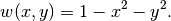
Practical values for an infinite
may be 50 or larger, and in such cases the program will report the
maximum deviation between the computed and the (approximate) exact
 .
.
Note that the variational formulation remains the same as in the
program from the section Implementation (1), except that is
replaced by and  .
The final program is found in the file membrane1.py, located
in the stationary/poisson directory, and also listed below.
We have inserted capabilities for iterative solution methods and
hence large meshes (the section Controlling the Solution Process),
used objects for the variational problem and solver
(the section Linear Variational Problem and Solver Objects), and made numerical
comparison of the numerical and (approximate) analytical solution
(the section Examining the Discrete Solution).
.
The final program is found in the file membrane1.py, located
in the stationary/poisson directory, and also listed below.
We have inserted capabilities for iterative solution methods and
hence large meshes (the section Controlling the Solution Process),
used objects for the variational problem and solver
(the section Linear Variational Problem and Solver Objects), and made numerical
comparison of the numerical and (approximate) analytical solution
(the section Examining the Discrete Solution).
"""
FEniCS program for the deflection w(x,y) of a membrane:
-Laplace(w) = p = Gaussian function, in a unit circle,
with w = 0 on the boundary.
"""
from dolfin import *
import numpy
# Set pressure function:
T = 10.0 # tension
A = 1.0 # pressure amplitude
R = 0.3 # radius of domain
theta = 0.2
x0 = 0.6*R*cos(theta)
y0 = 0.6*R*sin(theta)
sigma = 0.025
sigma = 50 # large value for verification
n = 40 # approx no of elements in radial direction
mesh = UnitCircle(n)
V = FunctionSpace(mesh, 'Lagrange', 1)
# Define boundary condition w=0
def boundary(x, on_boundary):
return on_boundary
bc = DirichletBC(V, Constant(0.0), boundary)
# Define variational problem
w = TrialFunction(V)
v = TestFunction(V)
a = inner(nabla_grad(w), nabla_grad(v))*dx
f = Expression('4*exp(-0.5*(pow((R*x[0] - x0)/sigma, 2)) '
' -0.5*(pow((R*x[1] - y0)/sigma, 2)))',
R=R, x0=x0, y0=y0, sigma=sigma)
L = f*v*dx
# Compute solution
w = Function(V)
problem = LinearVariationalProblem(a, L, w, bc)
solver = LinearVariationalSolver(problem)
solver.parameters['linear_solver'] = 'cg'
solver.parameters['preconditioner'] = 'ilu'
solver.solve()
# Plot scaled solution, mesh and pressure
plot(mesh, title='Mesh over scaled domain')
plot(w, title='Scaled deflection')
f = interpolate(f, V)
plot(f, title='Scaled pressure')
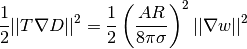
# Find maximum real deflection
max_w = w.vector().array().max()
max_D = A*max_w/(8*pi*sigma*T)
print 'Maximum real deflection is', max_D
# Verification for "flat" pressure (large sigma)
if sigma >= 50:
w_e = Expression("1 - x[0]*x[0] - x[1]*x[1]")
w_e = interpolate(w_e, V)
dev = numpy.abs(w_e.vector().array() - w.vector().array()).max()
print 'sigma=%g: max deviation=%e' % (sigma, dev)
# Should be at the end
interactive()
Choosing a small width (say 0.01) and a location
toward the circular boundary (say  for any
 ![\theta\in [0,2\pi]](_images/math/d496801364e2500716592c61aa49c79aa526f4ba.png) ), may produce an exciting visual
comparison of and that demonstrates the very smoothed elastic
response to a peak force (or mathematically, the smoothing properties
of the inverse of the Laplace operator). One needs to experiment with
the mesh resolution to get a smooth visual representation of~$f$. You
are strongly encouraged to play around with the plots and different
mesh resolutions.
), may produce an exciting visual
comparison of and that demonstrates the very smoothed elastic
response to a peak force (or mathematically, the smoothing properties
of the inverse of the Laplace operator). One needs to experiment with
the mesh resolution to get a smooth visual representation of~$f$. You
are strongly encouraged to play around with the plots and different
mesh resolutions.
As we go along with examples it is fun to play around with plot commands and visualize what is computed. This section explains some useful visualization features.
The plot(u) command launches a FEniCS component called Viper, which applies the VTK package to visualize finite element functions. Viper is not a full-fledged, easy-to-use front-end to VTK (like Mayavi2, ParaView or, VisIt), but rather a thin layer on top of VTK’s Python interface, allowing us to quickly visualize a DOLFIN function or mesh, or data in plain Numerical Python arrays, within a Python program. Viper is ideal for debugging, teaching, and initial scientific investigations. The visualization can be interactive, or you can steer and automate it through program statements. More advanced and professional visualizations are usually better done with advanced tools like Mayavi2, ParaView, or VisIt.
We have made a program membrane1v.py for the membrane deflection problem in the section Solving a Real Physical Problem and added various demonstrations of Viper capabilities. You are encouraged to play around with membrane1v.py and modify the code as you read about various features.
The plot function can take additional arguments, such as a title of the plot, or a specification of a wireframe plot (elevated mesh) instead of a colored surface plot:
plot(mesh, title='Finite element mesh')
plot(w, wireframe=True, title='solution')
The three mouse buttons can be used to rotate, translate, and zoom the surface. Pressing h in the plot window makes a printout of several key bindings that are available in such windows. For example, pressing m in the mesh plot window dumps the plot of the mesh to an Encapsulated PostScript (.eps) file, while pressing i saves the plot in PNG format. All plotfile names are automatically generated as simulationX.eps, where X is a counter 0000, 0001, 0002, etc., being increased every time a new plot file in that format is generated (the extension of PNG files is .png instead of .eps). Pressing o adds a red outline of a bounding box around the domain.
One can alternatively control the visualization from the program code
directly. This is done through a Viper object returned from
the plot command. Let us grab this object and use it to
1) tilt the camera  degrees in the latitude direction, 2) add
and axes, 3) change the default name of the plot files,
4) change the color scale, and 5) write the plot
to a PNG and an EPS file. Here is the code:
degrees in the latitude direction, 2) add
and axes, 3) change the default name of the plot files,
4) change the color scale, and 5) write the plot
to a PNG and an EPS file. Here is the code:
viz_w = plot(w,
            wireframe=False,
            title='Scaled membrane deflection',
            rescale=False,
            axes=True,              # include axes
            basename='deflection',  # default plotfile name
            )

viz_w.elevate(-65) # tilt camera -65 degrees (latitude dir)
viz_w.set_min_max(0, 0.5*max_w)  # color scale
viz_w.update(w)    # bring settings above into action
viz_w.write_png('deflection.png')
viz_w.write_ps('deflection', format='eps')
The format argument in the latter line can also take the values 'ps' for a standard PostScript file and 'pdf' for a PDF file. Note the necessity of the viz_w.update(w) call – without it we will not see the effects of tilting the camera and changing the color scale. Figure Plot of the deflection of a membrane shows the resulting scalar surface.
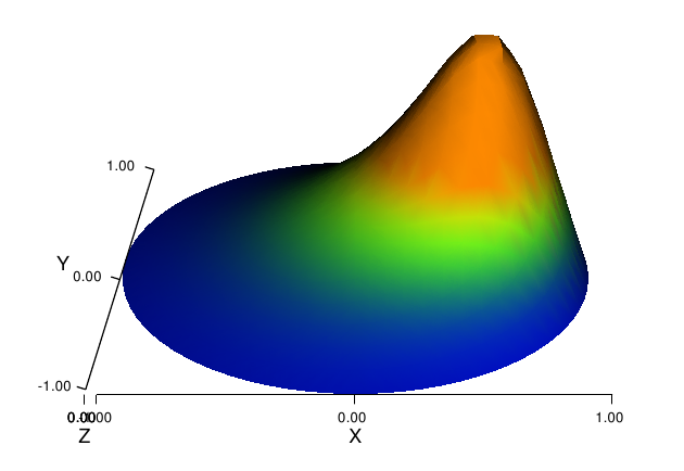
Plot of the deflection of a membrane
In Poisson and many other problems the gradient of the solution is
of interest. The computation is in principle simple:
since
 , we have that
Given the solution variable u in the program, its gradient is
obtained by grad(u) or nabla_grad(u).
However, the gradient of a piecewise continuous
finite element scalar field
is a discontinuous vector field
since the has discontinuous derivatives at the boundaries of
the cells. For example, using Lagrange elements of degree 1, is
linear over each cell, and the numerical becomes a piecewise
constant vector field. On the contrary,
the exact gradient is continuous.
For visualization and data analysis purposes
we often want the computed
gradient to be a continuous vector field. Typically,
we want each component of to be represented in the same
way as itself. To this end, we can project the components
of onto the
same function space as we used for .
This means that we solve  approximately by a finite element
method, using the same elements for the components of
as we used for . This process is known as projection.
approximately by a finite element
method, using the same elements for the components of
as we used for . This process is known as projection.
Looking at the component  of the gradient, we project the (discrete) derivative
 onto a function space
with basis
onto a function space
with basis  such that the derivative in
this space is expressed by the standard sum
such that the derivative in
this space is expressed by the standard sum  ,
for suitable (new) coefficients
,
for suitable (new) coefficients  .
.
The variational problem for reads: find  such that
where
The function spaces  and
and  (with the superscript
g denoting “gradient”) are
vector versions of the function space for , with
boundary conditions removed (if is the
space we used for , with no restrictions
on boundary values,
(with the superscript
g denoting “gradient”) are
vector versions of the function space for , with
boundary conditions removed (if is the
space we used for , with no restrictions
on boundary values, ![V^{(\mbox{g})} = \hat{V^{(\mbox{g})}} = [V]^d](_images/math/11a00d706aec5b98d443acab30242c68acb17f48.png) , where
is the number of space dimensions).
For example, if we used piecewise linear functions on the mesh to
approximate , the variational problem for corresponds to
approximating each component field of by piecewise linear functions.
, where
is the number of space dimensions).
For example, if we used piecewise linear functions on the mesh to
approximate , the variational problem for corresponds to
approximating each component field of by piecewise linear functions.
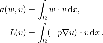
The variational problem for the vector field
, called grad_u in the code, is easy to solve in FEniCS:
V_g = VectorFunctionSpace(mesh, 'Lagrange', 1)
w = TrialFunction(V_g)
v = TestFunction(V_g)

a = inner(w, v)*dx
L = inner(grad(u), v)*dx
grad_u = Function(V_g)
solve(a == L, grad_u)

plot(grad_u, title='grad(u)')
The boundary condition argument to solve is dropped since there are no essential boundary conditions in this problem. The new thing is basically that we work with a VectorFunctionSpace, since the unknown is now a vector field, instead of the FunctionSpace object for scalar fields. Figure Example of visualizing the vector field by arrows at the nodes shows example of how Viper can visualize such a vector field.
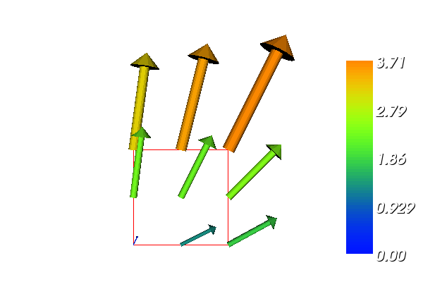
Example of visualizing the vector field by arrows at the nodes
The scalar component fields of the gradient can be extracted as separate fields and, e.g., visualized:
grad_u_x, grad_u_y = grad_u.split(deepcopy=True)  # extract components
plot(grad_u_x, title='x-component of grad(u)')
plot(grad_u_y, title='y-component of grad(u)')
The deepcopy=True argument signifies a deep copy, which is a general term in computer science implying that a copy of the data is returned. (The opposite, deepcopy=False, means a shallow copy, where the returned objects are just pointers to the original data.)
The grad_u_x and grad_u_y variables behave as Function objects. In particular, we can extract the underlying arrays of nodal values by
grad_u_x_array = grad_u_x.vector().array()
grad_u_y_array = grad_u_y.vector().array()
The degrees of freedom of the grad_u vector field can also be reached by
grad_u_array = grad_u.vector().array()
but this is a flat numpy array where the degrees of freedom
for the component of the gradient is stored in the first part, then the
degrees of freedom of the component, and so on.
The program d5_p2D.py extends the
code d5_p2D.py from the section Examining the Discrete Solution
with computations and visualizations of the gradient.
Examining the arrays grad_u_x_array
and grad_u_y_array, or looking at the plots of
grad_u_x and
grad_u_y, quickly reveals that
the computed grad_u field does not equal the exact
gradient  in this particular test problem where
 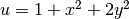 .
There are inaccuracies at the boundaries, arising from the
approximation problem for . Increasing the mesh resolution shows,
however, that the components of the gradient vary linearly as
.
There are inaccuracies at the boundaries, arising from the
approximation problem for . Increasing the mesh resolution shows,
however, that the components of the gradient vary linearly as
 and
and  in
the interior of the mesh (i.e., as soon as we are one element away from
the boundary). See the section Quick Visualization with VTK for illustrations of
this phenomenon.
in
the interior of the mesh (i.e., as soon as we are one element away from
the boundary). See the section Quick Visualization with VTK for illustrations of
this phenomenon.
Projecting some function onto some space is a very common operation in finite element programs. The manual steps in this process have therefore been collected in a utility function project(q, W), which returns the projection of some Function or Expression object named q onto the FunctionSpace or VectorFunctionSpace named W. Specifically, the previous code for projecting each component of grad(u) onto the same space that we use for u, can now be done by a one-line call
grad_u = project(grad(u), VectorFunctionSpace(mesh, 'Lagrange', 1))
The applications of projection are many, including turning discontinuous gradient fields into continuous ones, comparing higher- and lower-order function approximations, and transforming a higher-order finite element solution down to a piecewise linear field, which is required by many visualization packages.
Suppose we have a variable coefficient  in the Laplace operator,
as in the boundary-value problem
in the Laplace operator,
as in the boundary-value problem
(10)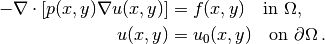
We shall quickly demonstrate that this simple extension of our model problem only requires an equally simple extension of the FEniCS program.
Let us continue to use our favorite solution 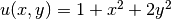 and
then prescribe
and
then prescribe 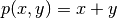 . It follows that
 and
and 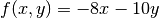 .
.
What are the modifications we need to do in the d4_p2D.py program from the section Examining the Discrete Solution?
- f must be an Expression since it is no longer a constant,
- a new Expression p must be defined for the variable coefficient,
- the variational problem is slightly changed.
First we address the modified variational problem. Multiplying
the PDE by a test function and
integrating by parts now results
in
The function spaces for and are the same as in
the section Variational Formulation, implying that the boundary integral
vanishes since on where we have Dirichlet conditions.
The weak form then has
In the code from the section Implementation (1) we must replace
a = inner(nabla_grad(u), nabla_grad(v))*dx
by
a = p*inner(nabla_grad(u), nabla_grad(v))*dx
The definitions of p and f read
p = Expression('x[0] + x[1]')
f = Expression('-8*x[0] - 10*x[1]')
No additional modifications are necessary. The complete code can be
found in in the file vcp2D.py (variable-coefficient Poisson problem in 2D).
You can run it and confirm
that it recovers the exact at the nodes.
The flux  may be of particular interest in
variable-coefficient Poisson problems as it often has an interesting
physical significance. As explained in the section Computing Derivatives,
we normally want the piecewise discontinuous flux or gradient to be
approximated by a continuous vector field, using the same elements as
used for the numerical solution . The approximation now consists of
solving
may be of particular interest in
variable-coefficient Poisson problems as it often has an interesting
physical significance. As explained in the section Computing Derivatives,
we normally want the piecewise discontinuous flux or gradient to be
approximated by a continuous vector field, using the same elements as
used for the numerical solution . The approximation now consists of
solving  by a finite element method: find
such that
by a finite element method: find
such that
where
This problem is identical to the one in the section Computing Derivatives,
except that enters the integral in .
The relevant Python statements for computing the flux field take the form
V_g = VectorFunctionSpace(mesh, 'Lagrange', 1)
w = TrialFunction(V_g)
v = TestFunction(V_g)

a = inner(w, v)*dx
L = inner(-p*grad(u), v)*dx
flux = Function(V_g)
solve(a == L, flux)
The following call to project is equivalent to the above statements:
flux = project(-p*grad(u),
               VectorFunctionSpace(mesh, 'Lagrange', 1))
Plotting the flux vector field is naturally as easy as plotting the gradient (see the section Computing Derivatives):
plot(flux, title='flux field')

flux_x, flux_y = flux.split(deepcopy=True)  # extract components
plot(flux_x, title='x-component of flux (-p*grad(u))')
plot(flux_y, title='y-component of flux (-p*grad(u))')
For data analysis of the nodal values of the flux field we can grab the underlying numpy arrays:
flux_x_array = flux_x.vector().array()
flux_y_array = flux_y.vector().array()
The program vcp2D.py contains in addition some plots,
including a curve plot
comparing flux_x and the exact counterpart along the line  .
The associated programming details related to this visualization
are explained in the section Visualization of Structured Mesh Data.
.
The associated programming details related to this visualization
are explained in the section Visualization of Structured Mesh Data.
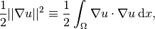
After the solution of a PDE is computed, we occasionally want to compute
functionals of , for example,
(11)
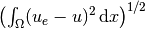
which often reflects some energy quantity. Another frequently occurring functional is the error
(12)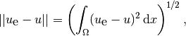
where is the exact solution. The error
is of particular interest when studying convergence properties.
Sometimes the interest concerns the flux out of a part  of
the boundary ,
of
the boundary ,
(13)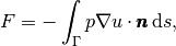
where  is an outward unit normal at and is a
coefficient (see the problem in the section A Variable-Coefficient Poisson Problem
for a specific example).
All these functionals are easy to compute with FEniCS, and this section
describes how it can be done.
is an outward unit normal at and is a
coefficient (see the problem in the section A Variable-Coefficient Poisson Problem
for a specific example).
All these functionals are easy to compute with FEniCS, and this section
describes how it can be done.
Energy Functional. The integrand of the
energy functional
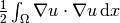 is described in the UFL language in the same manner as we describe
weak forms:
is described in the UFL language in the same manner as we describe
weak forms:
energy = 0.5*inner(grad(u), grad(u))*dx
E = assemble(energy)
The assemble call performs the integration. It is possible to restrict the integration to subdomains, or parts of the boundary, by using a mesh function to mark the subdomains as explained in the section Multiple Neumann, Robin, and Dirichlet Condition. The program membrane2.py carries out the computation of the elastic energy
in the membrane problem from the section Solving a Real Physical Problem.
Convergence Estimation. To illustrate error computations and convergence of finite element solutions, we modify the d5_p2D.py program from the section Computing Derivatives and specify a more complicated solution,

on the unit square.
This choice implies 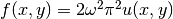 .
With
.
With  restricted to an integer
it follows that .
restricted to an integer
it follows that .
We need to define the
appropriate boundary conditions, the exact solution, and the function
in the code:
def boundary(x, on_boundary):
    return on_boundary

bc = DirichletBC(V, Constant(0.0), boundary)

omega = 1.0
u_e = Expression('sin(omega*pi*x[0])*sin(omega*pi*x[1])',
                 omega=omega)

f = 2*pi**2*omega**2*u_e
The computation of
 can be done by
error = (u - u_e)**2*dx
E = sqrt(assemble(error))
Here, u_e will be interpolated onto the function space V. This implies that the exact solution used in the integral will vary linearly over the cells, and not as a sine function, if V corresponds to linear Lagrange elements. This situation may yield a smaller error u - u_e than what is actually true.
More accurate representation of the exact solution is easily achieved by interpolating the formula onto a space defined by higher-order elements, say of third degree:
Ve = FunctionSpace(mesh, 'Lagrange', degree=3)
u_e_Ve = interpolate(u_e, Ve)
error = (u - u_e_Ve)**2*dx
E = sqrt(assemble(error))
To achieve complete mathematical control of which function space the computations are carried out in, we can explicitly interpolate u to the same space:
u_Ve = interpolate(u, Ve)
error = (u_Ve - u_e_Ve)**2*dx
The square in the expression for error will be expanded and lead to a lot of terms that almost cancel when the error is small, with the potential of introducing significant round-off errors. The function errornorm is available for avoiding this effect by first interpolating u and u_e to a space with higher-order elements, then subtracting the degrees of freedom, and then performing the integration of the error field. The usage is simple:
E = errornorm(u_e, u, normtype='L2', degree=3)
It is illustrative to look at the short implementation of errornorm:
def errornorm(u_e, u, Ve):
    u_Ve = interpolate(u, Ve)
    u_e_Ve = interpolate(u_e, Ve)
    e_Ve = Function(Ve)
    # Subtract degrees of freedom for the error field
    e_Ve.vector()[:] = u_e_Ve.vector().array() - \
                       u_Ve.vector().array()
    error = e_Ve**2*dx
    return sqrt(assemble(error))
The errornorm procedure turns out to be identical to computing the expression (u_e - u)**2*dx directly in the present test case.
Sometimes it is of interest to compute the error of the
gradient field:  (often referred to as the
  seminorm of the error).
Given the error field e_Ve above, we simply write
seminorm of the error).
Given the error field e_Ve above, we simply write
H1seminorm = sqrt(assemble(inner(grad(e_Ve), grad(e_Ve))*dx))
Finally, we remove all plot calls and printouts of values
in the original program, and
collect the computations in a function:
def compute(nx, ny, degree):
    mesh = UnitSquare(nx, ny)
    V = FunctionSpace(mesh, 'Lagrange', degree=degree)
    ...
    Ve = FunctionSpace(mesh, 'Lagrange', degree=5)
    E = errornorm(u_e, u, Ve)
    return E
Calling compute for finer and finer meshes enables us to
study the convergence rate. Define the element size
 , where
  is the number of divisions in and direction
(nx=ny in the code). We perform experiments with
is the number of divisions in and direction
(nx=ny in the code). We perform experiments with  and compute the corresponding errors
  and so forth.
Assuming
and so forth.
Assuming  for unknown constants
  and
and  , we can compare
two consecutive experiments, and
, we can compare
two consecutive experiments, and  ,
and solve for :
,
and solve for :
The values should approach the expected convergence
rate degree+1 as  increases.
The procedure above can easily be turned into Python code:
import sys
degree = int(sys.argv[1])  # read degree as 1st command-line arg
h = []  # element sizes
E = []  # errors
for nx in [4, 8, 16, 32, 64, 128, 264]:
    h.append(1.0/nx)
    E.append(compute(nx, nx, degree))

# Convergence rates
from math import log as ln  # (log is a dolfin name too - and logg :-)
for i in range(1, len(E)):
    r = ln(E[i]/E[i-1])/ln(h[i]/h[i-1])
    print 'h=%10.2E r=.2f'  (h[i], r)
The resulting program has the name d6_p2D.py
and computes error norms in various ways. Running this
program for elements of first degree and  yields the output
h=1.25E-01 E=3.25E-02 r=1.83
h=6.25E-02 E=8.37E-03 r=1.96
h=3.12E-02 E=2.11E-03 r=1.99
h=1.56E-02 E=5.29E-04 r=2.00
h=7.81E-03 E=1.32E-04 r=2.00
h=3.79E-03 E=3.11E-05 r=2.00
That is, we approach the expected second-order convergence of linear Lagrange elements as the meshes become sufficiently fine.
Running the program for second-degree elements results in the expected
value  ,
,
h=1.25E-01 E=5.66E-04 r=3.09
h=6.25E-02 E=6.93E-05 r=3.03
h=3.12E-02 E=8.62E-06 r=3.01
h=1.56E-02 E=1.08E-06 r=3.00
h=7.81E-03 E=1.34E-07 r=3.00
h=3.79E-03 E=1.53E-08 r=3.00
However, using (u - u_e)**2 for the error computation, which
implies interpolating u_e onto the same space as u,
results in  (!). This is an example where it is important to
interpolate u_e to a higher-order space (polynomials of
degree 3 are sufficient here) to avoid computing a too optimistic
convergence rate.
(!). This is an example where it is important to
interpolate u_e to a higher-order space (polynomials of
degree 3 are sufficient here) to avoid computing a too optimistic
convergence rate.
Running the program for third-degree elements results in the
expected value :
h=  1.25E-01 r=4.09
h=  6.25E-02 r=4.03
h=  3.12E-02 r=4.01
h=  1.56E-02 r=4.00
h=  7.81E-03 r=4.00
Checking convergence rates is the next best method for verifying PDE codes (the best being exact recovery of a solution as in the section Examining the Discrete Solution and many other places in this tutorial).
Flux Functionals. To compute flux integrals like
 we need to define the vector, referred to as facet normal
in FEniCS. If is the complete boundary we can perform
the flux computation by
we need to define the vector, referred to as facet normal
in FEniCS. If is the complete boundary we can perform
the flux computation by
n = FacetNormal(mesh)
flux = -p*dot(nabla_grad(u), n)*ds
total_flux = assemble(flux)
Although nabla_grad(u) and grad(u) are interchangeable in the above expression when u is a scalar function, we have chosen to write nabla_grad(u) because this is the right expression if we generalize the underlying equation to a vector Laplace/Poisson PDE. With grad(u) we must in that case write dot(n, grad(u)).
It is possible to restrict the integration to a part of the boundary using a mesh function to mark the relevant part, as explained in the section Multiple Neumann, Robin, and Dirichlet Condition. Assuming that the part corresponds to subdomain number i, the relevant form for the flux is -p*inner(grad(u), n)*ds(i).
When finite element computations are done on a structured rectangular mesh, maybe with uniform partitioning, VTK-based tools for completely unstructured 2D/3D meshes are not required. Instead we can use visualization and data analysis tools for structured data. Such data typically appear in finite difference simulations and image analysis. Analysis and visualization of structured data are faster and easier than doing the same with data on unstructured meshes, and the collection of tools to choose among is much larger. We shall demonstrate the potential of such tools and how they allow for tailored and flexible visualization and data analysis.
A necessary first step is to transform our mesh object to an object
representing a rectangle with equally-shaped rectangular cells. The
Python package scitools (code.google.com/p/scitools) has this
type of structure, called a UniformBoxGrid. The second step is to
transform the one-dimensional array of nodal values to a
two-dimensional array holding the values at the corners of the cells
in the structured grid. In such grids, we want to access a value by
its and indices, counting cells in the direction, and
counting cells in the direction. This transformation is in
principle straightforward, yet it frequently leads to obscure indexing
errors. The BoxField object in scitools takes conveniently care of
the details of the transformation. With a BoxField defined on a
UniformBoxGrid it is very easy to call up more standard plotting
packages to visualize the solution along lines in the domain or as 2D
contours or lifted surfaces.
Let us go back to the vcp2D.py code from the section A Variable-Coefficient Poisson Problem and map u onto a BoxField object:
import scitools.BoxField
u2 = u if u.ufl_element().degree() == 1 else \
     interpolate(u, FunctionSpace(mesh, 'Lagrange', 1))
u_box = scitools.BoxField.dolfin_function2BoxField(
        u2, mesh, (nx,ny), uniform_mesh=True)
The function dolfin_function2BoxField can only work with finite element fields with linear (degree 1) elements, so for higher-degree elements we here simply interpolate the solution onto a mesh with linear elements. We could also interpolate/project onto a finer mesh in the higher-degree case. Such transformations to linear finite element fields are very often needed when calling up plotting packages or data analysis tools. The u.ufl_element() method returns an object holding the element type, and this object has a method degree() for returning the element degree as an integer. The parameters nx and ny are the number of divisions in each space direction that were used when calling UnitSquare to make the mesh object. The result u_box is a BoxField object that supports “finite difference” indexing and an underlying grid suitable for numpy operations on 2D data. Also 1D and 3D meshes (with linear elements) can be turned into BoxField objects.
The ability to access a finite element field in the way one can access a finite difference-type of field is handy in many occasions, including visualization and data analysis. Here is an example of writing out the coordinates and the field value at a grid point with indices i and j (going from 0 to nx and ny, respectively, from lower left to upper right corner):
X = 0; Y = 1; Z = 0  # convenient indices

i = nx; j = ny   # upper right corner
print 'u(%g,%g)=%g' % (u_box.grid.coor[X][i],
                       u_box.grid.coor[Y][j],
                       u_box.values[i,j])
For instance,
the coordinates are reached by u_box.grid.coor[X].
The grid attribute is an instance of class UniformBoxGrid.
Many plotting programs can be used to visualize the data in u_box. Matplotlib is now a very popular plotting program in the Python world and could be used to make contour plots of u_box. However, other programs like Gnuplot, VTK, and MATLAB have better support for surface plots at the time of this writing. Our choice in this tutorial is to use the Python package scitools.easyviz, which offers a uniform MATLAB-like syntax as interface to various plotting packages such as Gnuplot, Matplotlib, VTK, OpenDX, MATLAB, and others. With scitools.easyviz we write one set of statements, close to what one would do in MATLAB or Octave, and then it is easy to switch between different plotting programs, at a later stage, through a command-line option, a line in a configuration file, or an import statement in the program. .. By default, scitools.easyviz employs Gnuplot as plotting program,
A contour plot is made by the following scitools.easyviz command:
import scitools.easyviz as ev
ev.contour(u_box.grid.coorv[X], u_box.grid.coorv[Y], u_box.values,
           5, clabels='on')
evtitle('Contour plot of u')
ev.savefig('u_contours.eps')

# or more compact syntax:
ev.contour(u_box.grid.coorv[X], u_box.grid.coorv[Y], u_box.values,
           5, clabels='on',
           savefig='u_contours.eps', title='Contour plot of u')
The resulting plot can be viewed in
Figure Finite element function on a structured 2D grid: contour plot of the solution.
The contour function needs arrays with the and coordinates
expanded to 2D arrays (in the same way as demanded when
making vectorized
numpy calculations of arithmetic expressions over all grid points).
The correctly expanded arrays are stored in grid.coorv.
The above call to
contour creates 5 equally spaced contour lines, and with
clabels='on' the contour values can be seen in the plot.
Other functions for visualizing 2D scalar fields are surf and mesh as known from MATLAB:
import scitools.easyviz as ev
ev.figure()
ev.surf(u_box.grid.coorv[X], u_box.grid.coorv[Y], u_box.values,
        shading='interp', colorbar='on',
        title='surf plot of u', savefig='u_surf.eps')

ev.figure()
ev.mesh(u_box.grid.coorv[X], u_box.grid.coorv[Y], u_box.values,
        title='mesh plot of u', savefig='u_mesh.eps')
Figure Finite element function on a structured 2D grid: surface plot of the solution and Finite element function on a structured 2D grid: lifted mesh plot of the solution exemplify the surfaces arising from the two plotting commands above. You can type pydoc scitools.easyviz in a terminal window to get a full tutorial. Note that scitools.easyviz offers function names like plot and mesh, which clash with plot from dolfin and the mesh variable in our programs. Therefore, we recommend the ev prefix.
A handy feature of BoxField is the ability to give a start point
in the grid and a direction, and then extract the field and corresponding
coordinates along the nearest grid
line. In 3D fields
one can also extract data in a plane.
Say we
want to plot along the line in the grid. The grid points,
x, and the
values along this line, uval, are extracted by
start = (0, 0.5)
x, uval, y_fixed, snapped = u_box.gridline(start, direction=X)
The variable snapped is true if the line had to be snapped onto a
gridline and in that case y_fixed holds the snapped
(altered) value.
Plotting versus the coordinate along this line, using
scitools.easyviz, is now a matter of
ev.figure()  # new plot window
ev.plot(x, uval, 'r-')  # 'r--: red solid line
ev.title('Solution')
ev.legend('finite element solution')

# or more compactly:
ev.plot(x, uval, 'r-', title='Solution',
        legend='finite element solution')
A more exciting plot compares the projected numerical flux in
direction along the
line with the exact flux:
ev.figure()
flux2_x = flux_x if flux_x.ufl_element().degree() == 1 else \
          interpolate(flux_x, FunctionSpace(mesh, 'Lagrange', 1))
flux_x_box = scitools.BoxField.dolfin_function2BoxField(
          flux2_x, mesh, (nx,ny), uniform_mesh=True)
x, fluxval, y_fixed, snapped = \
          flux_x_box.gridline(start, direction=X)
y = y_fixed
flux_x_exact = -(x + y)*2*x
ev.plot(x, fluxval, 'r-',
        x, flux_x_exact, 'b-',
        legend=('numerical (projected) flux', 'exact flux'),
        title='Flux in x-direction (at y=%g)' % y_fixed,
        savefig='flux.eps')
As seen from Figure Finite element function on a structured 2D grid: curve plot of the exact flux and the projected numerical flux, the numerical flux is accurate except in the boundary elements.
The visualization constructions shown above and used to generate the figures are found in the program vcp2D.py in the stationary/poisson directory.
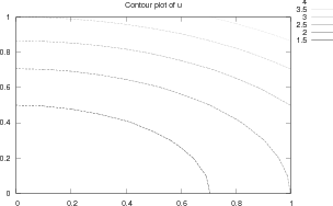
Finite element function on a structured 2D grid: contour plot of the solution
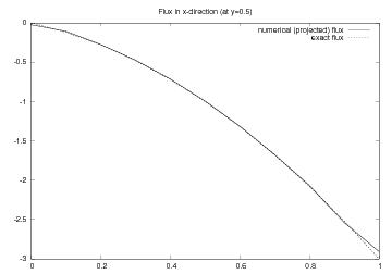
Finite element function on a structured 2D grid: curve plot of the exact flux and the projected numerical flux
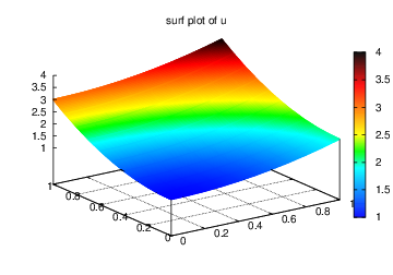
Finite element function on a structured 2D grid: surface plot of the solution
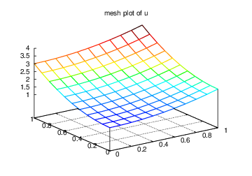
Finite element function on a structured 2D grid: lifted mesh plot of the solution
It should be easy with the information above to transform a finite element field over a uniform rectangular or box-shaped mesh to the corresponding BoxField object and perform MATLAB-style visualizations of the whole field or the field over planes or along lines through the domain. By the transformation to a regular grid we have some more flexibility than what Viper offers. However, we remark that comprehensive tools like VisIt, MayaVi2, or ParaView also have the possibility for plotting fields along lines and extracting planes in 3D geometries, though usually with less degree of control compared to Gnuplot, MATLAB, and Matplotlib. For example, in investigations of numerical accuracy or numerical artifacts one is often interested in studying curve plots where only the nodal values sampled. This is straightforward with a structured mesh data structure, but more difficult in visualization packages utilizing unstructured grids, as hitting exactly then nodes when sampling a function along a line through the grid might be non-trivial.
Let us make a slight extension of our two-dimensional Poisson problem
from the section The Poisson equation
and add a Neumann boundary condition. The domain is still
the unit square, but now we set the Dirichlet condition
at the left and right sides,
 and
and  , while the Neumann condition

is applied to the remaining
sides  and
and  .
The Neumann condition is also known as a natural boundary condition
(in contrast to an essential boundary condition).
.
The Neumann condition is also known as a natural boundary condition
(in contrast to an essential boundary condition).
Let  and
and  denote the parts of where the Dirichlet and Neumann
conditions apply, respectively.
The complete boundary-value problem can be written as
denote the parts of where the Dirichlet and Neumann
conditions apply, respectively.
The complete boundary-value problem can be written as
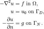
Again we choose  as the exact solution and adjust ,
  , and
accordingly:
, and
accordingly:
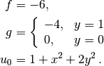
For ease of programming we may introduce a function defined over the whole
of such that takes on the right values at and
. One possible extension is
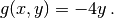
The first task is to derive the variational problem. This time we cannot
omit the boundary term arising from the integration by parts, because
is only zero on . We have
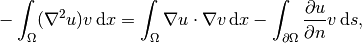
and since on ,
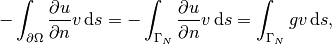
by applying the boundary condition on .
The resulting weak form reads
(14)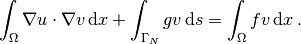
Expressing this equation
in the standard notation is straightforward with
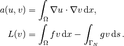
How does the Neumann condition impact the implementation? Starting with any of the previous files d*_p2D.py, say d4_p2D.py, we realize that the statements remain almost the same. Only two adjustments are necessary:
- The function describing the boundary where Dirichlet conditions apply must be modified.
- The new boundary term must be added to the expression in L.
Step 1 can be coded as
def Dirichlet_boundary(x, on_boundary):
    if on_boundary:
        if x[0] == 0 or x[0] == 1:
            return True
        else:
            return False
    else:
        return False
A more compact implementation reads
def Dirichlet_boundary(x, on_boundary):
    return on_boundary and (x[0] == 0 or x[0] == 1)
As pointed out already in the section Implementation (1), testing for an exact match of real numbers is not good programming practice so we introduce a tolerance in the test:
def Dirichlet_boundary(x, on_boundary):
    tol = 1E-14   # tolerance for coordinate comparisons
    return on_boundary and \
           (abs(x[0]) < tol or abs(x[0] - 1) < tol)
The second adjustment of our program concerns the definition of L,
where we have to add a boundary integral and a definition of the
function to be integrated:
g = Expression('-4*x[1]')
L = f*v*dx - g*v*ds
The ds variable implies a boundary integral, while dx
implies an integral over the domain .
No more modifications are necessary.
The file dn1_p2D.py in the stationary/poisson directory
implements this problem. Running the program verifies the implementation:
equals the exact solution at all the nodes,
regardless of how many elements we use.
The PDE problem from the previous section applies a function  for setting Dirichlet conditions at two parts of the boundary.
Having a single function to set multiple Dirichlet conditions is
seldom possible. The more general case is to have
for setting Dirichlet conditions at two parts of the boundary.
Having a single function to set multiple Dirichlet conditions is
seldom possible. The more general case is to have  functions for
setting Dirichlet conditions on parts of the boundary.
The purpose of this section is to explain how such multiple conditions
are treated in FEniCS programs.
functions for
setting Dirichlet conditions on parts of the boundary.
The purpose of this section is to explain how such multiple conditions
are treated in FEniCS programs.
Let us return to the case from the section Combining Dirichlet and Neumann Conditions and define two separate functions for the two Dirichlet conditions:
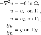
Here,  is the boundary , while
 corresponds to the boundary .
We have that
corresponds to the boundary .
We have that  ,
, 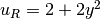 , and
, and  .
For the left boundary we
define
the usual triple of a function for the boundary value,
a function for defining
the boundary of interest, and a DirichletBC object:
.
For the left boundary we
define
the usual triple of a function for the boundary value,
a function for defining
the boundary of interest, and a DirichletBC object:
u_L = Expression('1 + 2*x[1]*x[1]')

def left_boundary(x, on_boundary):
    tol = 1E-14   # tolerance for coordinate comparisons
    return on_boundary and abs(x[0]) < tol

Gamma_0 = DirichletBC(V, u_L, left_boundary)
For the boundary we write a similar code snippet:
u_R = Expression('2 + 2*x[1]*x[1]')

def right_boundary(x, on_boundary):
    tol = 1E-14   # tolerance for coordinate comparisons
    return on_boundary and abs(x[0] - 1) < tol

Gamma_1 = DirichletBC(V, u_R, right_boundary)
The various essential conditions are then collected in a list and used in the solution process:
bcs = [Gamma_0, Gamma_1]
...
solve(a == L, u, bcs)
# or
problem = LinearVariationalProblem(a, L, u, bcs)
solver  = LinearVariationalSolver(problem)
solver.solve()
In other problems, where the values are constant at a part of the
boundary, we may use a simple Constant object instead of an
Expression object.
The file dn2_p2D.py contains a complete program which demonstrates the constructions above. An extended example with multiple Neumann conditions would have been quite natural now, but this requires marking various parts of the boundary using the mesh function concept and is therefore left to the section Multiple Neumann, Robin, and Dirichlet Condition.
Given , the discrete solution is computed by
inserting  into and demanding
to be fulfilled for
into and demanding
to be fulfilled for  test functions
 . This implies
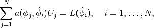
which is nothing but a linear system,

where the entries in and  are given by
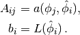
The examples so far have specified the left- and right-hand side
of the variational formulation and then asked FEniCS to
assemble the linear system and solve it.
An alternative to is explicitly call functions for assembling the
coefficient matrix and the right-side vector , and then solve
the linear system  with respect to the
  vector.
Instead of solve(a == L, u, bc) we now write
vector.
Instead of solve(a == L, u, bc) we now write
A = assemble(a)
b = assemble(L)
bc.apply(A, b)
u = Function(V)
U = u.vector()
solve(A, U, b)
The variables a and L are as before. That is, a refers to the
bilinear form involving a TrialFunction object (say u)
and a TestFunction object (v), and L involves a
TestFunction object (v). From a and L,
the assemble function can
compute and .
The matrix and vector are first assembled without incorporating
essential (Dirichlet) boundary conditions. Thereafter, the
call bc.apply(A, b) performs the necessary modifications of
the linear system such that u is guaranteed to equal the prescribed
boundary values.
When we have multiple Dirichlet conditions stored in a list bcs,
as explained in the section Multiple Dirichlet Conditions, we must apply
each condition in bcs to the system:
# bcs is a list of DirichletBC objects
for bc in bcs:
    bc.apply(A, b)
There is an alternative function assemble_system, which can assemble the system and take boundary conditions into account in one call:
A, b = assemble_system(a, L, bcs)
The assemble_system function incorporates the boundary conditions in the element matrices and vectors, prior to assembly. The conditions are also incorporated in a symmetric way to preserve eventual symmetry of the coefficient matrix. .. That is, for each degree of freedom
With bc.apply(A, b) the matrix A is modified in an unsymmetric way. .. : The row is zero’ed out
Note that the solution u is, as before, a Function object.
The degrees of freedom,  , are filled
into u‘s Vector object (u.vector())
by the solve function.
, are filled
into u‘s Vector object (u.vector())
by the solve function.
The object A is of type Matrix, while b and u.vector() are of type Vector. We may convert the matrix and vector data to numpy arrays by calling the array() method as shown before. If you wonder how essential boundary conditions are incorporated in the linear system, you can print out A and b before and after the bc.apply(A, b) call:
A = assemble(a)
b = assemble(L)
if mesh.num_cells() < 16:  # print for small meshes only
    print A.array()
    print b.array()
bc.apply(A, b)
if mesh.num_cells() < 16:
    print A.array()
    print b.array()
With access to the elements in A through a numpy array we can easily perform computations on this matrix, such as computing the eigenvalues (using the eig function in numpy.linalg). We can alternatively dump A and b to file in MATLAB format and invoke MATLAB or Octave to analyze the linear system. Dumping the arrays A and b to MATLAB format is done by
import scipy.io
scipy.io.savemat('Ab.mat', {'A': A.array(), 'b': b.array()})
Writing load Ab.mat in MATLAB or Octave will then make the variables A and b available for computations.
Matrix processing in Python or MATLAB/Octave is only feasible for small PDE problems since the numpy arrays or matrices in MATLAB file format are dense matrices. DOLFIN also has an interface to the eigensolver package SLEPc, which is a preferred tool for computing the eigenvalues of large, sparse matrices of the type encountered in PDE problems (see demo/la/eigenvalue in the DOLFIN source code tree for a demo).
A complete code where the linear system is explicitly assembled and
solved is found in the file dn3_p2D.py in the directory
stationary/poisson. This code solves the same problem as in
dn2_p2D.py
(the section Multiple Dirichlet Conditions). For small
linear systems, the program writes out A and b before and
after incorporation of essential boundary conditions and illustrates
the difference between assemble and assemble_system.
The reader is encouraged to run the code for a  mesh (UnitSquare(2, 1) and study the output of A.
By default, solve(A, U, b) applies sparse LU decomposition as solver. Specification of an iterative solver and preconditioner is done through two optional arguments:
solve(A, U, b, 'cg', 'ilu')
Appropriate names of solvers and preconditioners are found in the section Linear Solvers and Preconditioners.
To control tolerances in the stopping criterion and the maximum number of iterations, one can explicitly form a KrylovSolver object and set items in its parameters attribute (see also the section Linear Variational Problem and Solver Objects):
solver = KrylovSolver('cg', 'ilu')
solver.parameters['absolute_tolerance'] = 1E-7
solver.parameters['relative_tolerance'] = 1E-4
solver.parameters['maximum_iterations'] = 1000
u = Function(V)
U = u.vector()
set_log_level(DEBUG)
solver.solve(A, U, b)
The program dn4_p2D.py is a modification of dn3_p2D.py illustrating this latter approach.
The choice of start vector for the iterations in a linear solver is often
important. With the solver.solve(A, U, b) call the default start vector
is the zero vector. A start vector
with random numbers in the interval ![[-100,100]](_images/math/aa78ca392ad05ca27d7e044893984b4c71a74a0f.png) can be computed as
can be computed as
n = u.vector().array().size
U = u.vector()
U[:] = numpy.random.uniform(-100, 100, n)
solver.parameters['nonzero_initial_guess'] = True
solver.solve(A, U, b)
Note that we must turn off the default behavior of setting the start vector (“initial guess”) to zero. A random start vector is included in the dn4_p2D.py code.
Creating the linear system explicitly in a program can have some
advantages in more advanced problem settings. For example, may
be constant throughout a time-dependent simulation, so we can avoid
recalculating at every time level and save a significant amount
of simulation time. The sections Implementation (2)
and Avoiding Assembly deal with this topic
in detail.
FEniCS makes it is easy to write a unified simulation code that can
operate in 1D, 2D, and 3D. We will conveniently make use of this
feature in forthcoming examples. As an appetizer, go back to the
introductory program d1_p2D.py in the stationary/poisson directory
and change the mesh construction from UnitSquare(6, 4) to
UnitCube(6, 4, 5). Now the domain is the unit cube partitioned into
 boxes, and each box is divided into six
tetrahedra-shaped finite elements for computations. Run the program
and observe that we can solve a 3D problem without any other
modifications (!). The visualization allows you to rotate the cube and
observe the function values as colors on the boundary.
boxes, and each box is divided into six
tetrahedra-shaped finite elements for computations. Run the program
and observe that we can solve a 3D problem without any other
modifications (!). The visualization allows you to rotate the cube and
observe the function values as colors on the boundary.
The forthcoming material introduces some convenient technicalities such that the same program can run in 1D, 2D, or 3D without any modifications. Consider the simple model problem
![u''(x) = 2\hbox{ in }[0,1],\quad u(0)=0,\ u(1)=1,](_images/math/612751bf9d86487f9a1edd1eb6f27dceeb5c7d98.png)
with exact solution  . Our aim is to formulate and solve this
problem in a 2D and a 3D domain as well.
We may generalize the domain
. Our aim is to formulate and solve this
problem in a 2D and a 3D domain as well.
We may generalize the domain ![[0,1]](_images/math/e861e10e1c19918756b9c8b7717684593c63aeb8.png) to a rectangle or box of any size
in the and directions and pose homogeneous Neumann
conditions
to a rectangle or box of any size
in the and directions and pose homogeneous Neumann
conditions  at all additional boundaries
 and
and  to ensure that only varies with
. For example, let us choose
a unit hypercube as domain:
to ensure that only varies with
. For example, let us choose
a unit hypercube as domain: ![\Omega = [0,1]^d](_images/math/79b66cb050453a982a65155c90c482e80871b71a.png) , where is the number
of space dimensions. The generalized $d$-dimensional Poisson problem
then reads
, where is the number
of space dimensions. The generalized $d$-dimensional Poisson problem
then reads
(15)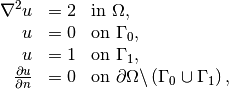
where is the side of the hypercube where , and
where is the side where .
Implementing a PDE for any is no more
complicated than solving a problem with a specific number of dimensions.
The only non-trivial part of the code is actually to define the mesh.
We use the command line for the user-input to the program. The first argument
can be the degree of the polynomial in the finite element basis functions.
Thereafter, we supply the
cell divisions in the various spatial directions. The number of
command-line arguments will then imply the number of space dimensions.
For example, writing 3 10 3 4 on the command line means that
we want to approximate by piecewise polynomials of degree 3,
and that the domain is a three-dimensional cube with  divisions in the , , and directions, respectively.
.. Each of the
divisions in the , , and directions, respectively.
.. Each of the  boxes will
The Python code can be quite compact:
degree = int(sys.argv[1])
divisions = [int(arg) for arg in sys.argv[2:]]
d = len(divisions)
domain_type = [UnitInterval, UnitSquare, UnitCube]
mesh = domain_type[d-1](*divisions)
V = FunctionSpace(mesh, 'Lagrange', degree)
First note that although sys.argv[2:] holds the divisions of the mesh, all elements of the list sys.argv[2:] are string objects, so we need to explicitly convert each element to an integer. The construction domain_type[d-1] will pick the right name of the object used to define the domain and generate the mesh. Moreover, the argument *divisions sends all the component of the list divisions as separate arguments. For example, in a 2D problem where divisions has two elements, the statement
mesh = domain_type[d-1](*divisions)
is equivalent to
mesh = UnitSquare(divisions[0], divisions[1])
The next part of the program is to set up the boundary conditions.
Since the Neumann conditions have  we can
omit the boundary integral from the weak form. We then only
need to take care of Dirichlet conditions at two sides:
we can
omit the boundary integral from the weak form. We then only
need to take care of Dirichlet conditions at two sides:
tol = 1E-14   # tolerance for coordinate comparisons
def Dirichlet_boundary0(x, on_boundary):
    return on_boundary and abs(x[0]) < tol

def Dirichlet_boundary1(x, on_boundary):
    return on_boundary and abs(x[0] - 1) < tol

bc0 = DirichletBC(V, Constant(0), Dirichlet_boundary0)
bc1 = DirichletBC(V, Constant(1), Dirichlet_boundary1)
bcs = [bc0, bc1]
Note that this code is independent of the number of space dimensions. So are the statements defining and solving the variational problem:
u = TrialFunction(V)
v = TestFunction(V)
f = Constant(-2)
a = inner(nabla_grad(u), nabla_grad(v))*dx
L = f*v*dx

u = Function(V)
solve(a == L, u, bcs)
The complete code is found in the file paD.py (Poisson problem in “anyD”).
If we want to parameterize the direction in which varies, say by
the space direction number e, we only need to replace x[0] in the
code by x[e]. The parameter e could be given as a second
command-line argument. The reader is encouraged to perform this
modification.